Excel ISBLANK Function: Learn with Example

What is ISBLANK function?

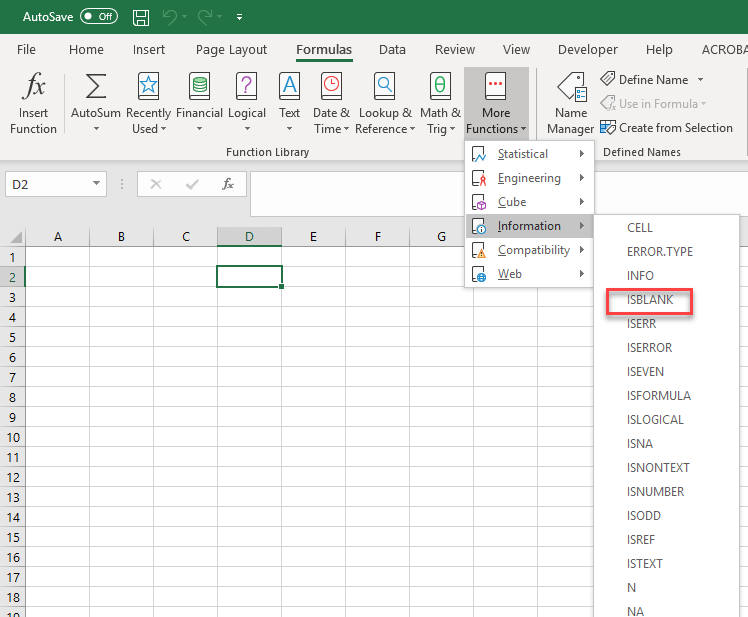
ISBLANK function used to check whether a cell is empty or not. Since this is an information function, it always returns a Boolean value, true or false. If the cell contains a value it will return false and true will be returned if it is not empty.

ISBLANK function in excel is grouped under information function. Information functions help to take a decision based on their results. You may come across a situation where you want to find the blank cells in an excel cell.

In this tutorial, you will learn:

• How to use the ISBLANK function?
• Example 1 How to use ISBLANK?
• Example 2: How to use ISBLANK with different excel functions?
• Example 3: How to use ISBLANK function with conditional formatting?

How to use the ISBLANK function?

Within a large range of cells when you want to find the blank cell ISBLANK function is the better option.

It is also used along with other functions and some formatting methods in Excel.

The formula for ISBLANK function

This is a simple function in excel, and the format is.

=ISBLANK(Value)

Where Value can be a cell reference

Example 1 How to use ISBLANK?

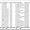
In following excel, given is the status of some orders. Order number and its delivery date are given. Let's find the orders which are not yet delivered.

Here you can consider the orders which do not have a delivery date marked can be considered as not yet delivered. So can apply the formula ISBLANK to find the blank cells in the column delivery_date.

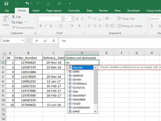
The format is '=ISBLANK(value)' for the value you can select the column delivery date corresponding to each order numbers.

So, the formula will be as given in the formula bar that is 'ISBLANK(C2)' where C2 refers to the delivery date of the first order.

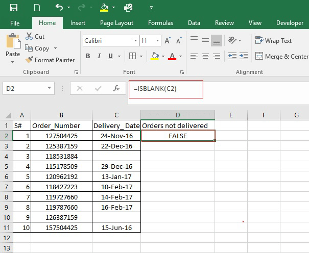
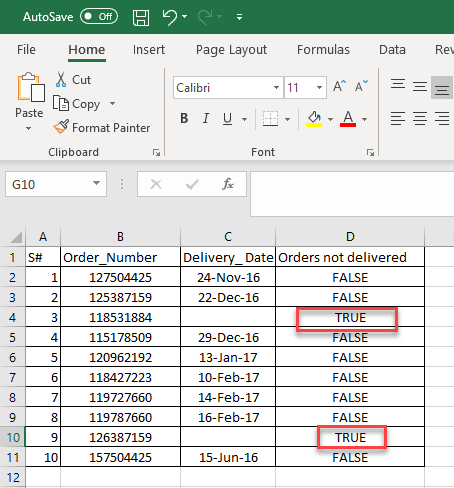
And the value returned as 'FALSE' since the delivery date is given which is a non-empty cell. You apply the same formula for the rest of the cells. For the order '118531884' delivery date is not given and the formula returns the result as 'TRUE.'

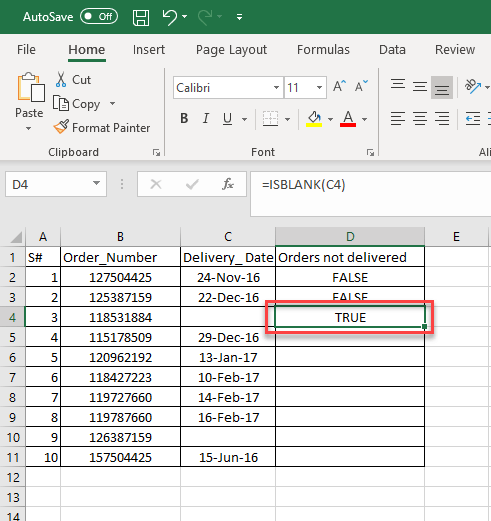
To find the undelivered orders applying the formula to each cell. For the orders '118531884, 126387159' delivery date is not given and is an empty cell. So, the ISBLANK function returns true. The delivery date which is true is the order not yet delivered.

Example 2: How to use ISBLANK with different excel functions?

In the above example, the ISBLANK function result gives TRUE or FALSE. The data is given below with order numbers and delivery date. In the status column, you want to get the result as 'complete' for orders which are delivered and 'No' for which are not delivered.

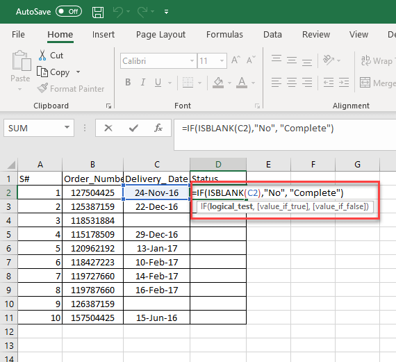
To get the results in the way you want, have to use some another function along with ISBLANK. IF function is used along with ISBLANK, to give result according to the two different conditions. If the cell is blank, it will return 'No' otherwise 'Complete.'

The formula applied is

=IF(ISBLANK(C2), "No", "Complete")

Here,

• the ISBLANK function will check the cell of delivery date, and according to the value, it will result in the true or false.
• This True/False is fed to the IF function that returns a 'No' if the cell is empty and statement 'Complete' if a value is present.

Here is the complete output

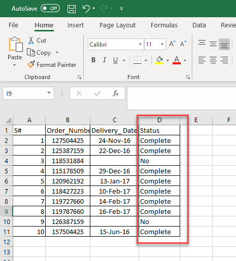
After applying the formula to the status of each order will get which are orders delivered and not delivered yet. Here the two orders are not completed the delivery rest are delivered.

Example 3: How to use ISBLANK function with conditional formatting?

ISBLANK function can be associated with conditional formatting to find blank cells and format the cells accordingly.

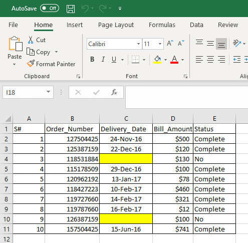
Step 1) Consider the following dataset that consists of data order_number, bill amount, delivery status. And you want to highlight the bill amount for which delivery is not completed.

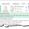
Step 2) Select the entire data, apply conditional formatting from the Home menu. Home->Conditional Formatting->New Rule

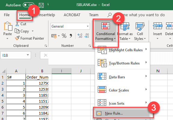
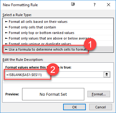
Step 3)

Select the option 'Use a formula to determine which cells to format.' This will allow you to insert a formula for a range of cells.

Give the formula '=ISBLANK($A$1:$E$11)' within the space.

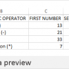
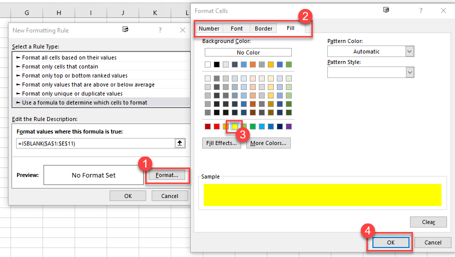
Step 4) Select the format which you want to apply to the cells from the format button.

1. By hitting the format button, you will get a dialogue window to select the format of the cells where the formula is applied.
2. Here, select the fill option to high light the formula applied cells where the condition matches.
3. Select the color you want to show
4. Hit the 'OK' button.

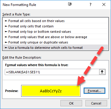
Step 5) Format will appear in the preview, click 'OK' button to apply.

Step 6) It will high light the blank cells after applying the ISBLANK formula with conditional formatting. Since the range value didn't work here, you have to apply the same rule for the entire column to get the result as below.

Download the Excel used in this Tutorial

Summary

• ISBLANK function will return a true or false value. True indicates the cell is blank.
• ISBLANK function can be used for conditional formatting as well as with other excel functions.
• An easy method to find blank cells within a large data set.
• Range of cells will not work with ISBLANK.