Data Warehousing
Star and Snowflake Schema in Data Warehouse with Examples
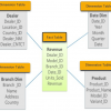
What is Multidimensional schema? Multidimensional Schema is especially designed to model data...
Pandas is an open-source library that allows to you perform data manipulation and analysis in Python. Pandas Python library offers data manipulation and data operations for numerical tables and time series. Pandas provide an easy way to create, manipulate, and wrangle the data. It is built on top of NumPy, means it needs NumPy to operate.
In this Python Pandas tutorial, you will learn Pandas Python basics like:
Data scientists make use of Pandas in Python for its following advantages:
In a nutshell, Pandas is a useful library in data analysis. It can be used to perform data manipulation and analysis. Pandas provide powerful and easy-to-use data structures, as well as the means to quickly perform operations on these structures.
Now in this Python Pandas tutorial, we will learn how to install Pandas in Python.
To install Pandas library, please refer our tutorial How to install TensorFlow. Pandas is installed by default. In remote case, pandas not installed-
You can install Pandas using:
import sys
!conda install --yes --prefix {sys.prefix} pandas Pandas DataFrame is a two-dimensional array with labelled data structure having different column types. A DataFrame is a standard way to store data in a tabular format, with rows to store the information and columns to name the information. For instance, the price can be the name of a column and 2,3,4 can be the price values.
Data Frame is well known by statistician and other data practitioners.
Below a picture of a Pandas data frame:

A series is a one-dimensional data structure. It can have any data structure like integer, float, and string. It is useful when you want to perform computation or return a one-dimensional array. A series, by definition, cannot have multiple columns. For the latter case, please use the data frame structure.
Python Pandas Series has following parameters:
pd.Series([1., 2., 3.])
0    1.0
1    2.0
2    3.0
dtype: float64
You can add the index with index. It helps to name the rows. The length should be equal to the size of the column
pd.Series([1., 2., 3.], index=['a', 'b', 'c'])
Below, you create a Pandas series with a missing value for the third rows. Note, missing values in Python are noted "NaN." You can use numpy to create missing value: np.nan artificially
pd.Series([1,2,np.nan])
Output
0    1.0
1    2.0
2    NaN
dtype: float64
Now in this Pandas DataFrame tutorial, we will learn how to create Python Pandas dataframe:
You can convert a numpy array to a pandas data frame with pd.Data frame(). The opposite is also possible. To convert a pandas Data Frame to an array, you can use np.array()
## Numpy to pandas
import numpy as np
h = [[1,2],[3,4]]
df_h = pd.DataFrame(h)
print('Data Frame:', df_h)

## Pandas to numpy
df_h_n = np.array(df_h)
print('Numpy array:', df_h_n)
Data Frame:    0  1
0  1  2
1  3  4
Numpy array: [[1 2]
 [3 4]]
You can also use a dictionary to create a Pandas dataframe.
dic = {'Name': ["John", "Smith"], 'Age': [30, 40]}
pd.DataFrame(data=dic) | Age | Name | |
|---|---|---|
| 0 | 30 | John |
| 1 | 40 | Smith |
Pandas have a convenient API to create a range of date. Let's learn with Python Pandas examples:
pd.data_range(date,period,frequency):
## Create date
# Days
dates_d = pd.date_range('20300101', periods=6, freq='D')
print('Day:', dates_d)
Output
Day: DatetimeIndex(['2030-01-01', '2030-01-02', '2030-01-03', '2030-01-04', '2030-01-05', '2030-01-06'], dtype='datetime64[ns]', freq='D')
# Months
dates_m = pd.date_range('20300101', periods=6, freq='M')
print('Month:', dates_m)
Output
Month: DatetimeIndex(['2030-01-31', '2030-02-28', '2030-03-31', '2030-04-30','2030-05-31', '2030-06-30'], dtype='datetime64[ns]', freq='M')
You can check the head or tail of the dataset with head(), or tail() preceded by the name of the panda's data frame as shown in the below Pandas example:
Step 1) Create a random sequence with numpy. The sequence has 4 columns and 6 rows
random = np.random.randn(6,4)
Step 2) Then you create a data frame using pandas.
Use dates_m as an index for the data frame. It means each row will be given a "name" or an index, corresponding to a date.
Finally, you give a name to the 4 columns with the argument columns
# Create data with date
df = pd.DataFrame(random,
                  index=dates_m,
                  columns=list('ABCD'))
Step 3) Using head function
df.head(3)
| A | B | C | D | |
|---|---|---|---|---|
| 2030-01-31 | 1.139433 | 1.318510 | -0.181334 | 1.615822 |
| 2030-02-28 | -0.081995 | -0.063582 | 0.857751 | -0.527374 |
| 2030-03-31 | -0.519179 | 0.080984 | -1.454334 | 1.314947 |
Step 4) Using tail function
df.tail(3)
| A | B | C | D | |
|---|---|---|---|---|
| 2030-04-30 | -0.685448 | -0.011736 | 0.622172 | 0.104993 |
| 2030-05-31 | -0.935888 | -0.731787 | -0.558729 | 0.768774 |
| 2030-06-30 | 1.096981 | 0.949180 | -0.196901 | -0.471556 |
Step 5) An excellent practice to get a clue about the data is to use describe(). It provides the counts, mean, std, min, max and percentile of the dataset.
df.describe()
| A | B | C | D | |
|---|---|---|---|---|
| count | 6.000000 | 6.000000 | 6.000000 | 6.000000 |
| mean | 0.002317 | 0.256928 | -0.151896 | 0.467601 |
| std | 0.908145 | 0.746939 | 0.834664 | 0.908910 |
| min | -0.935888 | -0.731787 | -1.454334 | -0.527374 |
| 25% | -0.643880 | -0.050621 | -0.468272 | -0.327419 |
| 50% | -0.300587 | 0.034624 | -0.189118 | 0.436883 |
| 75% | 0.802237 | 0.732131 | 0.421296 | 1.178404 |
| max | 1.139433 | 1.318510 | 0.857751 | 1.615822 |
The last point of this Python Pandas tutorial is about how to slice a pandas data frame.
You can use the column name to extract data in a particular column as shown in the below Pandas example:
## Slice
### Using name
df['A']

2030-01-31   -0.168655
2030-02-28    0.689585
2030-03-31    0.767534
2030-04-30    0.557299
2030-05-31   -1.547836
2030-06-30    0.511551
Freq: M, Name: A, dtype: float64
To select multiple columns, you need to use two times the bracket, [[..,..]]
The first pair of bracket means you want to select columns, the second pairs of bracket tells what columns you want to return.
df[['A', 'B']].
| A | B | |
|---|---|---|
| 2030-01-31 | -0.168655 | 0.587590 |
| 2030-02-28 | 0.689585 | 0.998266 |
| 2030-03-31 | 0.767534 | -0.940617 |
| 2030-04-30 | 0.557299 | 0.507350 |
| 2030-05-31 | -1.547836 | 1.276558 |
| 2030-06-30 | 0.511551 | 1.572085 |
You can slice the rows with :
The code below returns the first three rows
### using a slice for row
df[0:3]
| A | B | C | D | |
|---|---|---|---|---|
| 2030-01-31 | -0.168655 | 0.587590 | 0.572301 | -0.031827 |
| 2030-02-28 | 0.689585 | 0.998266 | 1.164690 | 0.475975 |
| 2030-03-31 | 0.767534 | -0.940617 | 0.227255 | -0.341532 |
The loc function is used to select columns by names. As usual, the values before the coma stand for the rows and after refer to the column. You need to use the brackets to select more than one column.
## Multi col
df.loc[:,['A','B']]
| A | B | |
|---|---|---|
| 2030-01-31 | -0.168655 | 0.587590 |
| 2030-02-28 | 0.689585 | 0.998266 |
| 2030-03-31 | 0.767534 | -0.940617 |
| 2030-04-30 | 0.557299 | 0.507350 |
| 2030-05-31 | -1.547836 | 1.276558 |
| 2030-06-30 | 0.511551 | 1.572085 |
There is another method to select multiple rows and columns in Pandas. You can use iloc[]. This method uses the index instead of the columns name. The code below returns the same data frame as above
df.iloc[:, :2]
| A | B | |
|---|---|---|
| 2030-01-31 | -0.168655 | 0.587590 |
| 2030-02-28 | 0.689585 | 0.998266 |
| 2030-03-31 | 0.767534 | -0.940617 |
| 2030-04-30 | 0.557299 | 0.507350 |
| 2030-05-31 | -1.547836 | 1.276558 |
| 2030-06-30 | 0.511551 | 1.572085 |
You can drop columns using pd.drop()
df.drop(columns=['A', 'C'])
| B | D | |
|---|---|---|
| 2030-01-31 | 0.587590 | -0.031827 |
| 2030-02-28 | 0.998266 | 0.475975 |
| 2030-03-31 | -0.940617 | -0.341532 |
| 2030-04-30 | 0.507350 | -0.296035 |
| 2030-05-31 | 1.276558 | 0.523017 |
| 2030-06-30 | 1.572085 | -0.594772 |
You can concatenate two DataFrame in Pandas. You can use pd.concat()
First of all, you need to create two DataFrames. So far so good, you are already familiar with dataframe creation
import numpy as np
df1 = pd.DataFrame({'name': ['John', 'Smith','Paul'],
                     'Age': ['25', '30', '50']},
                    index=[0, 1, 2])
df2 = pd.DataFrame({'name': ['Adam', 'Smith' ],
                     'Age': ['26', '11']},
                    index=[3, 4])
Finally, you concatenate the two DataFrame
df_concat = pd.concat([df1,df2])
df_concat
| Age | name | |
|---|---|---|
| 0 | 25 | John |
| 1 | 30 | Smith |
| 2 | 50 | Paul |
| 3 | 26 | Adam |
| 4 | 11 | Smith |
If a dataset can contain duplicates information use, `drop_duplicates` is an easy to exclude duplicate rows. You can see that `df_concat` has a duplicate observation, `Smith` appears twice in the column `name.`
df_concat.drop_duplicates('name')| Age | name | |
|---|---|---|
| 0 | 25 | John |
| 1 | 30 | Smith |
| 2 | 50 | Paul |
| 3 | 26 | Adam |
You can sort value with sort_values
df_concat.sort_values('Age')| Age | name | |
|---|---|---|
| 4 | 11 | Smith |
| 0 | 25 | John |
| 3 | 26 | Adam |
| 1 | 30 | Smith |
| 2 | 50 | Paul |
You can use rename to rename a column in Pandas. The first value is the current column name and the second value is the new column name.
df_concat.rename(columns={"name": "Surname", "Age": "Age_ppl"})| Age_ppl | Surname | |
|---|---|---|
| 0 | 25 | John |
| 1 | 30 | Smith |
| 2 | 50 | Paul |
| 3 | 26 | Adam |
| 4 | 11 | Smith |
Below is a summary of the most useful method for data science with Pandas
| import data | read_csv |
|---|---|
| create series | Series |
| Create Dataframe | DataFrame |
| Create date range | date_range |
| return head | head |
| return tail | tail |
| Describe | describe |
| slice using name | dataname['columnname'] |
| Slice using rows | data_name[0:5] |
What is Multidimensional schema? Multidimensional Schema is especially designed to model data...
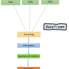
What is Information? Information is a set of data that is processed in a meaningful way according to...
With many Continuous Integration tools available in the market, it is quite a tedious task to...
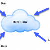
What is Data Lake? A Data Lake is a storage repository that can store large amount of structured,...
Data mining is looking for hidden, valid, and all the possible useful patterns in large size data...
Tableau Server is designed in a way to connect many data tiers. It can connect clients from...