DevOps

What is ITSM? IT Service Management Processes, Framework, Benefits
What is ITSM? ITSM aims to align the delivery of IT services with the needs of the enterprise. The...
In this tutorial, you will learn:
Following are the Data Types or Data Structures in R Programming:
Basics types
We can check the type of a variable with the class function
Example 1:
# Declare variables of different types
# Numeric
x <- 28
class(x)
Output:
## [1] "numeric"
Example 2:
# String
y <- "R is Fantastic"
class(y)
Output:
## [1] "character"
Example 3:
# Boolean
z <- TRUE
class(z)
Output:
## [1] "logical"
Variables are one of the basic data types in R that store values and are an important component in R programming, especially for a data scientist. A variable in R data types can store a number, an object, a statistical result, vector, dataset, a model prediction basically anything R outputs. We can use that variable later simply by calling the name of the variable.
To declare variable data structures in R, we need to assign a variable name. The name should not have space. We can use _ to connect to words.
To add a value to the variable in data types in R programming, use <- or =.
Here is the syntax:
# First way to declare a variable:  use the `<-`
name_of_variable <- value
# Second way to declare a variable:  use the `=`
name_of_variable = value
In the command line, we can write the following codes to see what happens:
Example 1:
# Print variable x
x <- 42
x
Output:
## [1] 42
Example 2:
y  <- 10
y
Output:
## [1] 10
Example 3:
# We call x and y and apply a subtraction
x-y
Output:
## [1] 32
A vector is a one-dimensional array. We can create a vector with all the basic R data types we learnt before. The simplest way to build vector data structures in R, is to use the c command.
Example 1:
# Numerical
vec_num <- c(1, 10, 49)
vec_num
Output:
## [1] 1 10 49
Example 2:
# Character
vec_chr <- c("a", "b", "c")
vec_chr
Output:
## [1] "a" "b" "c"
Example 3:
# Boolean
vec_bool <-  c(TRUE, FALSE, TRUE)
vec_bool
Output:
##[1] TRUE FALSE TRUE
We can do arithmetic calculations on vector binary operators in R.
Example 4:
# Create the vectors
vect_1 <- c(1, 3, 5)
vect_2 <- c(2, 4, 6)
# Take the sum of A_vector and B_vector
sum_vect <- vect_1 + vect_2
# Print out total_vector
sum_vect
Output:
[1] 3 7 11
Example 5:
In R, it is possible to slice a vector. In some occasion, we are interested in only the first five rows of a vector. We can use the [1:5] command to extract the value 1 to 5.
# Slice the first five rows of the vector
slice_vector <- c(1,2,3,4,5,6,7,8,9,10)
slice_vector[1:5]
Output:
## [1] 1 2 3 4 5
Example 6:
The shortest way to create a range of value is to use the: between two numbers. For instance, from the above example, we can write c(1:10) to create a vector of value from one to ten.
# Faster way to create adjacent values
c(1:10)
Output:
## [1] 1 2 3 4 5 6 7 8 9 10
We will first see the basic arithmetic operators in R data types. Following are the arithmetic and boolean operators in R programming which stand for:
Operator | Description |
|---|---|
| + | Addition |
| - | Subtraction |
| * | Multiplication |
| / | Division |
| ^ or ** | Exponentiation |
Example 1:
# An addition
3 + 4
Output:
## [1] 7
You can easily copy and paste the above R code into Rstudio Console. The output is displayed after the character #. For instance, we write the code print('gtupapers') the output will be ##[1] gtupapers.
The ## means we print an output and the number in the square bracket ([1]) is the number of the display
The sentences starting with # annotation. We can use # inside an R script to add any comment we want. R won't read it during the running time.
Example 2:
# A multiplication
3*5
Output:
## [1] 15
Example 3:
# A division
(5+5)/2
Output:
## [1] 5
Example 4:
# Exponentiation
2^5
Output:
Example 5:
## [1] 32
# Modulo
28%%6
Output:
## [1] 4
With logical operators, we want to return values inside the vector based on logical conditions. Following is a detailed list of logical operators of data types in R programming
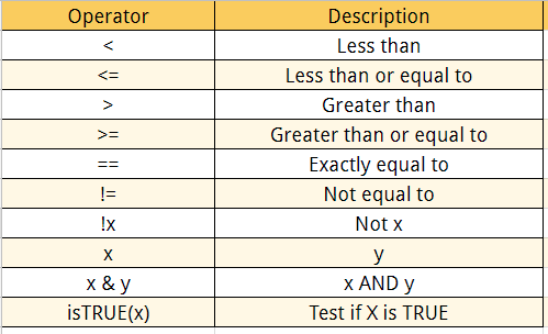
The logical statements in R are wrapped inside the []. We can add many conditional statements as we like but we need to include them in a parenthesis. We can follow this structure to create a conditional statement:
variable_name[(conditional_statement)]
With variable_name referring to the variable, we want to use for the statement. We create the logical statement i.e. variable_name > 0. Finally, we use the square bracket to finalize the logical statement. Below, an example of a logical statement.
Example 1:
# Create a vector from 1 to 10
logical_vector <- c(1:10)
logical_vector>5
Output:
## [1]FALSE FALSE FALSE FALSE FALSE TRUE TRUE TRUE TRUE TRUE
In the output above, R reads each value and compares it to the statement logical_vector>5. If the value is strictly superior to five, then the condition is TRUE, otherwise FALSE. R returns a vector of TRUE and FALSE.
Example 2:
In the example below, we want to extract the values that only meet the condition 'is strictly superior to five'. For that, we can wrap the condition inside a square bracket precede by the vector containing the values.
# Print value strictly above 5
logical_vector[(logical_vector>5)]
Output:
## [1] 6 7 8 9 10
Example 3:
# Print 5 and 6
logical_vector <- c(1:10)
logical_vector[(logical_vector>4) & (logical_vector<7)]
Output:
## [1] 5 6
What is ITSM? ITSM aims to align the delivery of IT services with the needs of the enterprise. The...
Off-cycle Payroll runs are used to make payments outside the regular payroll run like one time...
Who is a Software Developer? Software developers are professional who builds software which runs...
What is Cucumber? Cucumber is a testing tool that supports Behavior Driven Development (BDD). It...
OS Tutorial Summary This Operating System Tutorial offers all the basic and advanced concepts of...
What is Dependency Injection in AngularJS? Dependency Injection is a software design pattern that...