Python

BEST Python Certification Exam in 2021
What is Python Certification? Python certification training courses help you to master the...
SciPy in Python is an open-source library used for solving mathematical, scientific, engineering, and technical problems. It allows users to manipulate the data and visualize the data using a wide range of high-level Python commands. SciPy is built on the Python NumPy extention. SciPy is also pronounced as "Sigh Pi."
Sub-packages of SciPy:
In this tutorial, you will learn:
Numpy:
SciPy:
You can also install SciPy in Windows via pip
Python3 -m pip install --user numpy scipy
Install Scipy on Linux
sudo apt-get install python-scipy python-numpy
Install SciPy in Mac
sudo port install py35-scipy py35-numpy
Before start to learning SciPy, you need to know basic functionality as well as different types of an array of NumPy
The standard way of import infSciPy modules and Numpy:
from scipy import special   #same for other modules
import numpy as np
Scipy, I/O package, has a wide range of functions for work with different files format which are Matlab, Arff, Wave, Matrix Market, IDL, NetCDF, TXT, CSV and binary format.
Let's we take one file format example as which are regularly use of MatLab:
 import numpy as np
 from scipy import io as sio
 array = np.ones((4, 4))
 sio.savemat('example.mat', {'ar': array})
 data = sio.loadmat(‘example.mat', struct_as_record=True)
 data['ar']
Output:
array([[ 1., 1., 1., 1.],
           [ 1., 1., 1., 1.],
           [ 1., 1., 1., 1.],
           [ 1., 1., 1., 1.]])
Code Explanation
help(scipy.special)
Output :
NAME
    scipy.special

DESCRIPTION
    ========================================
    Special functions (:mod:`scipy.special`)
    ========================================

    .. module:: scipy.special

    Nearly all of the functions below are universal functions and follow
    broadcasting and automatic array-looping rules. Exceptions are noted.
Cubic Root function finds the cube root of values.
Syntax:
scipy.special.cbrt(x)
Example:
from scipy.special import cbrt
#Find cubic root of 27 & 64 using cbrt() function
cb = cbrt([27, 64])
#print value of cb
print(cb)
Output: array([3., 4.])
Exponential function computes the 10**x element-wise.
Example:
from scipy.special import exp10
#define exp10 function and pass value in its
exp = exp10([1,10])
print(exp)
Output: [1.e+01 1.e+10]
SciPy also gives functionality to calculate Permutations and Combinations.
Combinations - scipy.special.comb(N,k)
Example:
from scipy.special import comb
#find combinations of 5, 2 values using comb(N, k)
com = comb(5, 2, exact = False, repetition=True)
print(com)
Output: 15.0
Permutations –
scipy.special.perm(N,k)
Example:
from scipy.special import perm
#find permutation of 5, 2 using perm (N, k) function
per = perm(5, 2, exact = True)
print(per)
Output: 20
Log Sum Exponential computes the log of sum exponential input element.
Syntax :
scipy.special.logsumexp(x)
Nth integer order calculation function
Syntax :
scipy.special.jn()
Now let's do some test with scipy.linalg,
Calculating determinant of a two-dimensional matrix,
from scipy import linalg
import numpy as np
#define square matrix
two_d_array = np.array([ [4,5], [3,2] ])
#pass values to det() function
linalg.det( two_d_array )
Output: -7.0
Inverse Matrix –
scipy.linalg.inv()
Inverse Matrix of Scipy calculates the inverse of any square matrix.
Let's see,
from scipy import linalg
import numpy as np
# define square matrix
two_d_array = np.array([ [4,5], [3,2] ])
#pass value to function inv()
linalg.inv( two_d_array )
Output:
array( [[-0.28571429,  0.71428571],
       [ 0.42857143, -0.57142857]] )
Eigenvalues and Eigenvector – scipy.linalg.eig()
Example,
from scipy import linalg
import numpy as np
#define two dimensional array
arr = np.array([[5,4],[6,3]])
#pass value into function
eg_val, eg_vect = linalg.eig(arr)
#get eigenvalues
print(eg_val)
#get eigenvectors
print(eg_vect)
Output:
[ 9.+0.j -1.+0.j] #eigenvalues
 [ [ 0.70710678 -0.5547002 ] #eigenvectors
   [ 0.70710678  0.83205029] ]
Example: Take a wave and show using Matplotlib library. we take simple periodic function example of sin(20 × 2πt)
%matplotlib inline
from matplotlib import pyplot as plt
import numpy as np

#Frequency in terms of Hertz
fre  = 5
#Sample rate
fre_samp = 50
t = np.linspace(0, 2, 2 * fre_samp, endpoint = False )
a = np.sin(fre  * 2 * np.pi * t)
figure, axis = plt.subplots()
axis.plot(t, a)
axis.set_xlabel ('Time (s)')
axis.set_ylabel ('Signal amplitude')
plt.show()
Output :
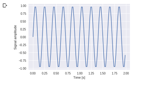
You can see this. Frequency is 5 Hz and its signal repeats in 1/5 seconds – it's call as a particular time period.
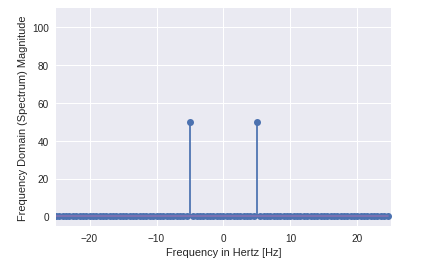
Now let us use this sinusoid wave with the help of DFT application.
from scipy import fftpack

A = fftpack.fft(a)
frequency = fftpack.fftfreq(len(a)) * fre_samp
figure, axis = plt.subplots()

axis.stem(frequency, np.abs(A))
axis.set_xlabel('Frequency in Hz')
axis.set_ylabel('Frequency Spectrum Magnitude')
axis.set_xlim(-fre_samp / 2, fre_samp/ 2)
axis.set_ylim(-5, 110)
plt.show()
Output:
%matplotlib inline
import matplotlib.pyplot as plt
from scipy import optimize
import numpy as np
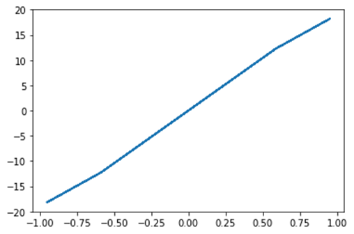
def function(a):
return a*2 + 20 * np.sin(a)
plt.plot(a, function(a))
plt.show()
#use BFGS algorithm for optimization
optimize.fmin_bfgs(function, 0)
Output:
Optimization terminated successfully.
Current function value: -23.241676
Iterations: 4
Function evaluations: 18
Gradient evaluations: 6
array([-1.67096375])
optimize.basinhopping(function, 0)
Output:
fun: -23.241676238045315
 lowest_optimization_result:
      fun: -23.241676238045315
 hess_inv: array([[0.05023331]])
      jac: array([4.76837158e-07])
  message: 'Optimization terminated successfully.'
     nfev: 15
      nit: 3
     njev: 5
   status: 0
  success: True
        x: array([-1.67096375])
                    message: ['requested number of basinhopping iterations completed successfully']
      minimization_failures: 0
                       nfev: 1530
                        nit: 100
                       njev: 510
               x: array([-1.67096375])
import numpy as np
from scipy.optimize import minimize
#define function f(x)
def f(x):
    return .4*(1 - x[0])**2

optimize.minimize(f, [2, -1], method="Nelder-Mead")
Output:
final_simplex: (array([[ 1.        , -1.27109375],
       [ 1.        , -1.27118835],
       [ 1.        , -1.27113762]]), array([0., 0., 0.]))
           fun: 0.0
       message: 'Optimization terminated successfully.'
          nfev: 147
           nit: 69
        status: 0
       success: True
             x: array([ 1.        , -1.27109375])
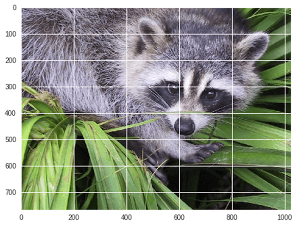
Example: Let's take a geometric transformation example of images
from scipy import misc
from matplotlib import pyplot as plt
import numpy as np
#get face image of panda from misc package
panda = misc.face()
#plot or show image of face
plt.imshow( panda )
plt.show()
Output:
Now we Flip-down current image:
#Flip Down using scipy misc.face image
flip_down = np.flipud(misc.face())
plt.imshow(flip_down)
plt.show()
Output:

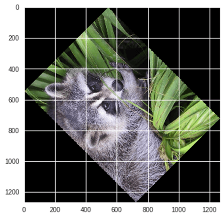
Example: Rotation of Image using Scipy,
from scipy import ndimage, misc
from matplotlib import pyplot as plt
panda = misc.face()
#rotatation function of scipy for image – image rotated 135 degree
panda_rotate = ndimage.rotate(panda, 135)
plt.imshow(panda_rotate)
plt.show()
Output:
Example: Now take an example of Single Integration

Here a is the upper limit and b is the lower limit
from scipy import integrate
# take f(x) function as f
f = lambda x : x**2
#single integration with a = 0 & b = 1
integration = integrate.quad(f, 0 , 1)
print(integration)
Output:
(0.33333333333333337, 3.700743415417189e-15)
Here function returns two values, in which the first value is integration and second value is estimated error in integral.
Example: Now take an example of double integration. We find the double integration of the following equation,
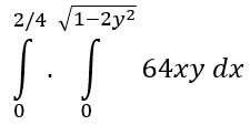
from scipy import integrate
import numpy as np
#import square root function from math lib
from math import sqrt
# set  fuction f(x)
f = lambda x, y : 64 *x*y
# lower limit of second integral
p = lambda x : 0
# upper limit of first integral
q = lambda y : sqrt(1 - 2*y**2)
# perform double integration
integration = integrate.dblquad(f , 0 , 2/4,  p, q)
print(integration)
Output:
(3.0, 9.657432734515774e-14)
You have seen that above output as same previous one.
| Package Name | Description |
|---|---|
| scipy.io |
|
| scipy.special |
|
| scipy.linalg |
|
| scipy.interpolate |
|
| scipy.optimize |
|
| scipy.stats |
|
| scipy.integrate |
|
| scipy.fftpack |
|
| scipy.signal |
|
| scipy.ndimage |
|
What is Python Certification? Python certification training courses help you to master the...
The following best online Python courses will help you to learn Python programming from home....
What is PyQt? PyQt is a python binding of the open-source widget-toolkit Qt, which also functions as...
Python count The count() is a built-in function in Python. It will return the total count of a...
What is Python Matrix? A Python matrix is a specialized two-dimensional rectangular array of data...
Python is one of the most popular programming languages. Currently, each of the following six...